Pymob in minutes - the basics#
This guide provides a streamlined introduction to the basic Pymob workflow and its key functionalities.
We will explore a simple linear regression model that we want to fit to a noisy dataset.
Pymob supports the modeling process by providing several tools for data structuring, parameter estimation and visualization of results.
If you are looking for a more detailed introduction, click here.
If you want to learn how to work with ODE models, check out this tutorial.
Pymob components 🧩#
Before starting the modeling process, let’s take a look at the main steps and modules of pymob:
Simulation:
First, we need to initialize a Simulation object by creating an instance of thepymob.simulation.SimulationBaseclass from the simulation module.
Optionally, we can configure the simulation withsim.config.case_study.name = "linear-regression",sim.config.case_study.scenario = "test"and many other options.Model:
Our model will be defined as a standard python function.
We will then assign it to the Simulation object by accessing the.modelattribute.Observations:
Our observation data must be structured as an xarray.Dataset.
We assign it to theobservationsattribute of our Simulation object.
Callingsim.config.data_structurewill give us further information about the layout of our data.Solver:
A solver (solvers) is required to solve the model.
In our simple case, we will use thesolve_analytic_1dsolver from theanalyticmodule.
We assign it to our Simulation object using thesolverattribute.
Since our model already provides an analytical solution, this solver basically does nothing. It is still needed to fulfill Pymob’s requirement for a solver component.
For more complex models (e.g. ODEs), theJaxSolverfrom thediffraxmodule is a more powerful option.
Users can also implement custom solvers as a subclass ofpymob.solvers.base.SolverBase.Inferer:
The inferer handels the parameter estimation.
Pymob supports various backends. In this example, we will work with NumPyro.
We assign the inferer to our Simulation object via theinfererattribute and configure the desired kernel (e.g. nuts).
But before inference, we need to parameterize our model using theParamclass.
Each parameter can be marked either as free or fixed, depending on whether it should be variable during the optimization procedure.
The parameters are stored in themodel_parametersdictionary, which holds model input values. By default, it takes the keys:parameters,y0andx_in.Evaluator:
The Evaluator is an instance to manage model evaluations. It sets up tasks, coordinates parallel runs of the simulation and keeps track of the results from each simulation or parameter inference process.
Evaluators store the raw output from a simulation and can generate an xarray object from it that corresponds to the data-structure of the observations with theresultsproperty. This automatically aligns the simulations results with the observations, for simple computation of loss functions.Config:
The simulation settings will be saved in a.cfgconfiguration file.
The config file contains information about our simulation in various sections. Learn more here.
We can further use it to create new simulations by loading settings from a config file.

Getting started 🛫#
# First, import the necessary python packages
import numpy as np
import matplotlib.pyplot as plt
import xarray as xr

# Import the pymob modules
from pymob.simulation import SimulationBase
from pymob.sim.solvetools import solve_analytic_1d
from pymob.sim.config import Param
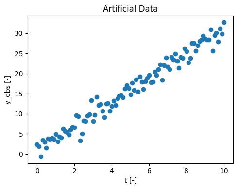
Since no measured data is provided, we will generate an artificial dataset.
\(y_{obs}\) represents the observed data over the time \(t\) [0, 10].
To use this data later in the simulation, we need to convert it into an xarray dataset.
In your own application, you would replace this with your measured experimental data.
# Parameter for the artificial data generation
rng = np.random.default_rng(seed=1)  # for reproducibility
slope = rng.uniform(2,4)
intercept = 1.0
num_points = 101
noise_level = 1.7

# generating time values
t = np.linspace(0, 10, num_points)

# generating y-values with noise
noise = rng.normal(0, noise_level, num_points)
y_obs = slope * t + intercept + noise

# visualizing our data
fig, ax = plt.subplots(figsize=(5, 4))
ax.scatter(t, y_obs, label='Datapoints')
ax.set(xlabel='t [-]', ylabel='y_obs [-]', title ='Artificial Data')
plt.tight_layout()

# convert the data to an xr-Dataset
data_obs = xr.DataArray(y_obs, coords={"t": t}).to_dataset(name="y")
data_obs
<xarray.Dataset>
Dimensions:  (t: 101)
Coordinates:
t (t) float64 0.0 0.1 0.2 0.3 0.4 0.5 … 9.5 9.6 9.7 9.8 9.9 10.0 Data variables: y (t) float64 2.397 1.864 -0.6106 3.446 … 27.91 31.2 29.83 32.7
Initialize a simulation ✨#
In pymob, a simulation object is initialized by creating an instance of the SimulationBase class from the simulation module.
We will choose a linear regression model, as it provides a good approximation of the data: \( y = a + b*x \)
x-dimension
The x_dimension of our simulation can have any name, for example t as often used for time series data.
You can specify it via sim.config.simulation.x_dimension.
# Initialize the Simulation object
sim = SimulationBase()

# configurate the case study
sim.config.case_study.name = "superquickstart"
sim.config.case_study.scenario = "linreg"

# Define the linear regression model
def linreg(x, a, b):
    return a + b * x

# Add the model to the simulation
sim.model = linreg

# Adding our dataset to the simulation
sim.observations = data_obs

# Defining a solver
sim.solver = solve_analytic_1d

# Take a look at the layut of the data
sim.config.data_structure
MinMaxScaler(variable=y, min=-0.6106386438473108, max=32.702588647741905)


/home/docs/checkouts/readthedocs.org/user_builds/pymob/envs/latest/lib/python3.11/site-packages/pymob/sim/config/base.py:397: UserWarning: Case study 'unnamed_case_study' could not be imported. Install the case study with `pip install unnamed_case_study`.
  warnings.warn(
/home/docs/checkouts/readthedocs.org/user_builds/pymob/envs/latest/lib/python3.11/site-packages/pymob/simulation.py:366: UserWarning: `sim.config.data_structure.y = Datavariable(dimensions=['t'] unit=None min=-0.6106386438473108 max=32.702588647741905 observed=True dimensions_evaluator=None)` has been assumed from `sim.observations`. If the order of the dimensions should be different, specify `sim.config.data_structure.y = DataVariable(dimensions=[...], ...)` manually.
  warnings.warn(


Datastructure(indices=[], y=DataVariable(dimensions=['t'], unit=None, min=-0.6106386438473108, max=32.702588647741905, observed=True, dimensions_evaluator=None))
Scalers
We notice a mysterious Scaler message. This tells us that our data variable has been identified and a scaler was constructed, which transforms the variable between [0, 1].
This has no effect at the moment, but it can be used later. Scaling can be powerful to help parameter estimation in more complex models.
Parameterizing and running the model 🏃#
Next, we define the model parameters \(a\) and \(b\).
Parameter \(a\) is set as fixed (free = False), meaning its value is known and will not be estimated during optimization.
Parameter \(b\) is marked as free (free = True), allowing it to be optimized to fit the data. As an initial guess, we assume \(b = 3\).
# Parameterizing the model
sim.config.model_parameters.a = Param(value=1.0, free=False)
sim.config.model_parameters.b = Param(value=3.0, free=True)
# this makes sure the model parameters are available to the model.
sim.model_parameters["parameters"] = sim.config.model_parameters.value_dict

sim.model_parameters["parameters"]
{'a': 1.0, 'b': 3.0}
Our model is now prepared with a defined parameter set.
To initialize the Evaluator, we call dispatch_constructor().
This step is essential and must be executed every time changes are made to the model.
The returned dataset (evaluator.results) has the exact same shape as the observation data.
# put everything in place for running the simulation
sim.dispatch_constructor()

# run
evaluator = sim.dispatch(theta={"b":3})
evaluator()
evaluator.results
/home/docs/checkouts/readthedocs.org/user_builds/pymob/envs/latest/lib/python3.11/site-packages/pymob/simulation.py:723: UserWarning: The number of ODE states was not specified in the config file [simulation] > 'n_ode_states = <n>'. Extracted the return arguments ['a+b*x'] from the source code. Setting 'n_ode_states=1.
  warnings.warn(
<xarray.Dataset>
Dimensions:  (t: 101)
Coordinates:
t (t) float64 0.0 0.1 0.2 0.3 0.4 0.5 … 9.5 9.6 9.7 9.8 9.9 10.0 Data variables: y (t) float64 1.0 1.3 1.6 1.9 2.2 2.5 … 29.8 30.1 30.4 30.7 31.0
What does the dispatch constructor do?
Behind the scenes, the dispatch constructor assembles a lightweight Evaluator object from the Simulation object, that takes the least necessary amount of information, runs it through some dimension checks, and also connects it to the specified solver and initializes it.
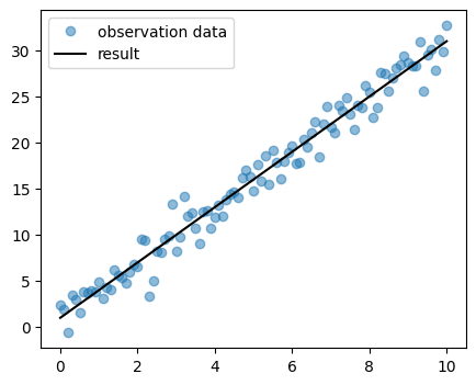
Let’s take a look at the results.
You can vary the parameter \(b\) in the previous step to investigate its influence on the model fit.
In the Introduction, you can try out the manual parameter estimation, which is a feature provided by Pymob.
fig, ax = plt.subplots(figsize=(5, 4))
data_res = evaluator.results
ax.plot(data_obs.t, data_obs.y, ls="", marker="o", color="tab:blue", alpha=.5, label ="observation data")
ax.plot(data_res.t, data_res.y, color="black", label ="result")
ax.legend()
<matplotlib.legend.Legend at 0x77fc11c5fc90>
Estimating parameters and uncertainty with MCMC 🤔#
Of course this example is very simple. In fact, we could optimize the parameters perfectly by hand.
But just for fun, let’s use Markov Chain Monte Carlo (MCMC) to estimate the parameters, their uncertainty and the uncertainty in the data.
We’ll run the parameter estimation with our inferer, using the NumPyro backend with a NUTS kernel. This completes the job in a few seconds.
We are almost ready to infer the model parameters. To also estimate the uncertainty of the parameters, we add another parameter representing the error and assume that it follows a lognormal distribution.
Additionally, we specify an error model for the data distribution. This will be: $\(y_{obs} \sim Normal (y, \sigma_y)\)$
Since \(\sigma_y\) is not a fixed parameter, it doesn’t need to be passed to the simulation class.
sim.config.model_parameters.sigma_y = Param(free=True , prior="lognorm(scale=1,s=1)", min=0, max=1)
sim.config.model_parameters.b.prior = "lognorm(scale=1,s=1)"
sim.config.error_model.y = "normal(loc=y,scale=sigma_y)"
sim.set_inferer("numpyro")
sim.inferer.config.inference_numpyro.kernel = "nuts"
sim.inferer.run()
# you can access the posterior distrubution by:
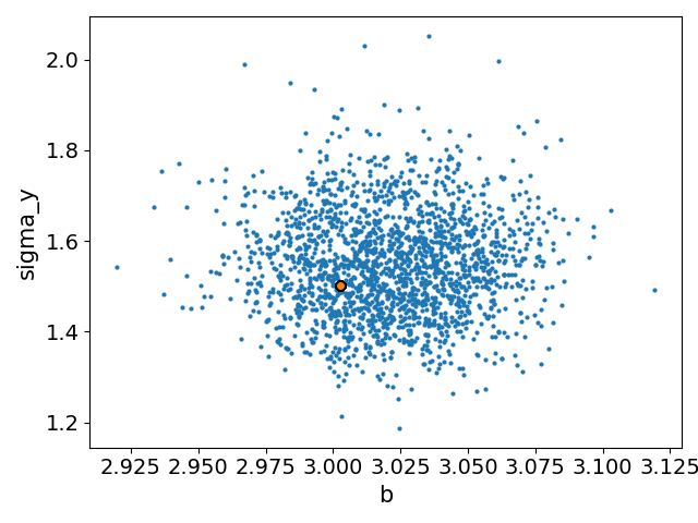
sim.inferer.idata.posterior
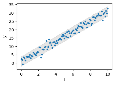
# Plot the results
sim.config.simulation.x_dimension = "t"
sim.posterior_predictive_checks(pred_hdi_style={"alpha": 0.1})
Jax 64 bit mode: False
Absolute tolerance: 1e-07


/home/docs/checkouts/readthedocs.org/user_builds/pymob/envs/latest/lib/python3.11/site-packages/pymob/inference/numpyro_backend.py:565: UserWarning: Model is not rendered, because the graphviz executable is not found. Try search for 'graphviz executables not found' and the used OS. This should be an easy fix :-)
  warnings.warn(


Trace Shapes:
 Param Sites:
Sample Sites:
       b dist     |
        value     |
 sigma_y dist     |
        value     |
   y_obs dist 101 |
        value 101 |
0%| | 0/3000 [00:00<?, ?it/s]
warmup: 0%| | 1/3000 [00:01<1:09:30, 1.39s/it, 1 steps of size 1.87e+00. acc. prob=0.00]
warmup: 14%|█▍ | 435/3000 [00:01<00:06, 404.91it/s, 3 steps of size 1.15e+00. acc. prob=0.79]
warmup: 29%|██▉ | 874/3000 [00:01<00:02, 872.91it/s, 3 steps of size 1.05e+00. acc. prob=0.79]
sample: 44%|████▍ | 1313/3000 [00:01<00:01, 1378.17it/s, 3 steps of size 8.42e-01. acc. prob=0.93]
sample: 59%|█████▊ | 1757/3000 [00:01<00:00, 1899.16it/s, 3 steps of size 8.42e-01. acc. prob=0.92]
sample: 73%|███████▎ | 2200/3000 [00:01<00:00, 2393.88it/s, 7 steps of size 8.42e-01. acc. prob=0.92]
sample: 88%|████████▊ | 2641/3000 [00:01<00:00, 2833.03it/s, 7 steps of size 8.42e-01. acc. prob=0.92]
sample: 100%|██████████| 3000/3000 [00:02<00:00, 1447.78it/s, 1 steps of size 8.42e-01. acc. prob=0.92]
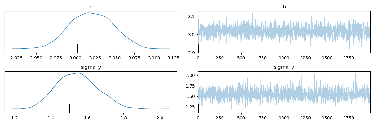
                mean       std    median      5.0%     95.0%     n_eff     r_hat
         b      3.00      0.03      3.00      2.96      3.04   1642.48      1.00
   sigma_y      1.47      0.10      1.46      1.29      1.63   1231.36      1.01

Number of divergences: 0
numpyro distributions
Currently only few distributions are implemented in the numpyro backend. This API will soon change, so that basically any distribution can be used to specifcy parameters.
We can inspect our estimates and see that the model provides a good fit for the parameters.
Note that we only get an estimate for \(b\). Previously, we set the parameter \(a\) with the flag free = False.
This effectively excludes it from the estimation and uses its default value, which was set to the true value a = 0.
Customize the posterior predictive checks
You can explore the API of pymob.sim.plot.SimulationPlot to find out how you can work on the default predictions. Of course you can always make your own plot, by accessing pymob.simulation.inferer.idata and pymob.simulation.observations
Report the results 🗒️#
Pymob provides the option to generate an automated report of the parameter distribution for a simulation.
The report can be configured by modifying the options in report().
# report the results
sim.report()
[WARNING] Could not fetch resource 'probability_model.png': replacing image with description
[WARNING] This document format requires a nonempty <title> element.
  Defaulting to 'report' as the title.
  To specify a title, use 'title' in metadata or --metadata title="...".
Exporting the simulation and running it via the case study API 📤#
After constructing the simulation, all settings - custom and default - can be exported to a comprehensive configuration file.
The simulation will be saved to the default path (CASE_STUDY/scenarios/SCENARIO/settings.cfg) or to a custom path, specified with the file path keyword fp.
Setting force=True will overwrite any existing config file, which is a reasonable choice in most cases.
From this point on, the simulation is (almost) ready to be executed from the command-line.
import os
sim.config.create_directory("scenario", force=True)
sim.config.create_directory("results", force=True)

# usually we expect to have a data directory in the case
os.makedirs(sim.data_path, exist_ok=True)
sim.save_observations(force=True)
sim.config.save(force=True)
Scenario directory created at '/home/docs/checkouts/readthedocs.org/user_builds/pymob/checkouts/latest/docs/source/user_guide/case_studies/superquickstart/scenarios/linreg'.
Results directory exists at '/home/docs/checkouts/readthedocs.org/user_builds/pymob/checkouts/latest/docs/source/user_guide/case_studies/superquickstart/results/linreg'.
Commandline API#
The command-line API runs a series of commands that load the case study, execute the initialize() method and perform some more initialization tasks before running the required job.
pymob-inferruns an inference job, for example:pymob-infer --case_study=quickstart --scenario=test --inference_backend=numpyro.
While there are more command-line options, these two (–case_study and –scenario) are required.