RNA pulse 5 substance independent#
The model RNA-pulse describes the damage dynamic as a expression pulse. It uses a sigmoid function to model the threshold dependent activation of Nrf2 expression and a concentration dependent exponential decay of RNA molecules. Coupled with active metabolization of the internal concentration of the chemical this leads to a pulse like behavior. In addition Nrf2 serves as a proxy for toxicodynamic damage
💥 Attention#
When calculating treatment effects it should be made sure that effects are calculated differentially to the initial value of the RNA expression
When \(R_0 \neq 1\), the RNA expression has to be divided by the baseline to obtain fold-change values, after the ODE has been solved.
Imports#
First, I apply some modifications to the jupyter notebook for a cleaner experience. Warnigns are ignored, the root directory is changed to the base of the repository. Then relevant packages are imported for the case study and its evaluation
import os
import json
import warnings
from functools import partial

import numpy as np
import arviz as az
import matplotlib as mpl
from matplotlib import pyplot as plt

from pymob import Config
from tktd_rna_pulse.sim import SingleSubstanceSim3

warnings.filterwarnings("ignore")
config = Config(config="../scenarios/rna_pulse_5_substance_independent_rna_protein_module/settings.cfg")
# change the package directory, because working in a jupyter notebook sets the root to the folder of the working directory
# the package gives the base directory of the case-study
config.case_study.package = "../.."
sim = SingleSubstanceSim3(config)
sim.setup()
MinMaxScaler(variable=cint, min=0.0, max=6364.836264471382)
MinMaxScaler(variable=nrf2, min=0.0, max=3.806557074337876)
MinMaxScaler(variable=survival, min=0.0, max=18.0)
Results directory exists at '/home/flo-schu/projects/hierarchical_tktd/case_studies/tktd_rna_pulse/results/rna_pulse_5_substance_independent_rna_protein_module'.
Scenario directory exists at '/home/flo-schu/projects/hierarchical_tktd/case_studies/tktd_rna_pulse/scenarios/rna_pulse_5_substance_independent_rna_protein_module'.
Parameter inference#
Parameter inference estimates the value of the parameters given the data presented to the model.
Here we calculate a maximum a posteriori (MAP) estimate which is the mode of the posterior distribution.
# set up the inferer properly
sim.set_inferer("numpyro")
Jax 64 bit mode: False
Absolute tolerance: 1e-06
First of all prior predictions are generated. These are helpful to diagnose
the model and also to compare posterior parameter estimates with the prior
distributions. If there is a large bias, this information can help to achieve
a better model fit. We can speed up the prior predictive sampling, if we let
the model only sample the prior distributions only_prior=True
# prior predictions
seed = 1
prior_predictions = sim.inferer.prior_predictions(n=100, seed=seed)
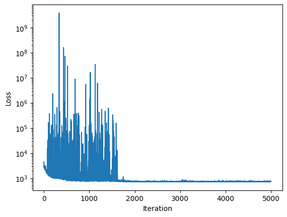
In the next step, we take the full model, including deterministic ODE solution and error model and run our SVI estimator on it, with the parameters that have been setup before.
# set the inference model
sim.config.inference_numpyro.kernel = "svi"
sim.config.inference_numpyro.svi_iterations = "5000"
sim.config.inference_numpyro.svi_learning_rate = "0.01"
sim.inferer.run()
                  Trace Shapes:
                   Param Sites:
                  Sample Sites:
 k_i_substance_normal_base dist      3 |
                          value      3 |
 k_m_substance_normal_base dist      3 |
                          value      3 |
z_ci_substance_normal_base dist      3 |
                          value      3 |
          r_rt_normal_base dist        |
                          value        |
          r_rd_normal_base dist        |
                          value        |
          v_rt_normal_base dist        |
                          value        |
           k_p_normal_base dist        |
                          value        |
           h_b_normal_base dist        |
                          value        |
             z_normal_base dist        |
                          value        |
            kk_normal_base dist        |
                          value        |
    sigma_cint_normal_base dist        |
                          value        |
    sigma_nrf2_normal_base dist        |
                          value        |
                  cint_obs dist 202 23 |
                          value 202 23 |
                  nrf2_obs dist 202 23 |
                          value 202 23 |
              survival_obs dist 202 23 |
                          value 202 23 |


100%|██████████| 5000/5000 [02:20<00:00, 35.66it/s, init loss: 4456.1201, avg. loss [4751-5000]: 737.9221]
arviz - WARNING - Shape validation failed: input_shape: (1, 1000), minimum_shape: (chains=2, draws=4)


                                mean     sd    hdi_3%   hdi_97%  mcse_mean  \
ci_max[101_0]               1757.000  0.000  1757.000  1757.000      0.000
ci_max[101_1]               1757.000  0.000  1757.000  1757.000      0.000
ci_max[106_0]               1757.000  0.000  1757.000  1757.000      0.000
ci_max[106_1]               1757.000  0.000  1757.000  1757.000      0.000
ci_max[112_0]               1757.000  0.000  1757.000  1757.000      0.000
...                              ...    ...       ...       ...        ...
z_ci[66_5]                     0.749  0.060     0.640     0.867      0.002
z_ci[6_0]                      0.749  0.060     0.640     0.867      0.002
z_ci_substance[diuron]         0.860  0.091     0.691     1.030      0.003
z_ci_substance[diclofenac]     0.687  0.065     0.568     0.811      0.002
z_ci_substance[naproxen]       0.749  0.060     0.640     0.867      0.002

                            mcse_sd  ess_bulk  ess_tail  r_hat
ci_max[101_0]                 0.000    1000.0    1000.0    NaN
ci_max[101_1]                 0.000    1000.0    1000.0    NaN
ci_max[106_0]                 0.000    1000.0    1000.0    NaN
ci_max[106_1]                 0.000    1000.0    1000.0    NaN
ci_max[112_0]                 0.000    1000.0    1000.0    NaN
...                             ...       ...       ...    ...
z_ci[66_5]                    0.001    1044.0     872.0    NaN
z_ci[6_0]                     0.001    1044.0     872.0    NaN
z_ci_substance[diuron]        0.002    1069.0     919.0    NaN
z_ci_substance[diclofenac]    0.001    1087.0     920.0    NaN
z_ci_substance[naproxen]      0.001    1044.0     872.0    NaN

[829 rows x 9 columns]
# show (and explore idata)
print(sim.inferer.idata)
Inference data with groups:
	> posterior
	> posterior_predictive
	> log_likelihood
	> observed_data
	> unconstrained_posterior
	> posterior_model_fits
	> posterior_residuals
	> posterior
	> posterior_predictive
	> log_likelihood
	> observed_data
	> posterior_model_fits
	> posterior_residuals
sim.inferer.store_results(f"{sim.output_path}/numpyro_svi_posterior.nc")
Posterior predictions#
In order to evaluate the goodness of fit for the posteriors, we are looking at the posterior predictions.
In order to obtain smoother trajectories, the time resolution is increased, and posterior predictions are calculated.
sim.coordinates["time"] = np.linspace(24, 120, 100)
sim.dispatch_constructor()
seed = int(np.random.random_integers(0, 100, 1))

res = sim.inferer.posterior_predictions(n=1, seed=seed).mean(("draw", "chain"))
print(res)
Posterior predictions: 100%|██████████| 1/1 [00:05<00:00,  5.95s/it]

<xarray.Dataset>
Dimensions:          (id: 202, time: 100)
Coordinates:
  * id               (id) object '101_0' '101_1' '106_0' ... '66_4' '66_5' '6_0'
  * time             (time) float64 24.0 24.97 25.94 26.91 ... 118.1 119.0 120.0
    hpf              (id) float64 24.0 24.0 24.0 24.0 ... 24.0 24.0 24.0 24.0
    nzfe             (id) float64 nan nan nan nan nan ... 9.0 9.0 9.0 9.0 20.0
    treatment_id     (id) int64 101 101 106 106 112 112 118 ... 66 66 66 66 66 6
    experiment_id    (id) int64 36 36 36 36 36 36 36 36 ... 27 27 27 27 27 27 1
    substance        (id) <U10 'diuron' 'diuron' ... 'naproxen' 'naproxen'
    substance_index  (id) int64 0 0 0 0 0 0 0 0 0 0 0 ... 2 2 2 2 2 2 2 2 2 2 2
    cluster          int64 0
Data variables:
    cext             (id, time) float32 2.34 2.34 2.34 ... 349.5 349.5 349.5
    cint             (id, time) float32 0.0 21.08 42.14 ... 3.177e+03 3.14e+03
    nrf2             (id, time) float32 1.0 1.016 1.031 ... 2.732 2.704 2.676
    P                (id, time) float32 0.0 7.153e-05 ... 0.8806 0.8877
    H                (id, time) float32 0.0 0.0001154 0.0002309 ... 1.804 1.822
    survival         (id, time) float32 1.0 0.9999 0.9998 ... 0.1646 0.1617
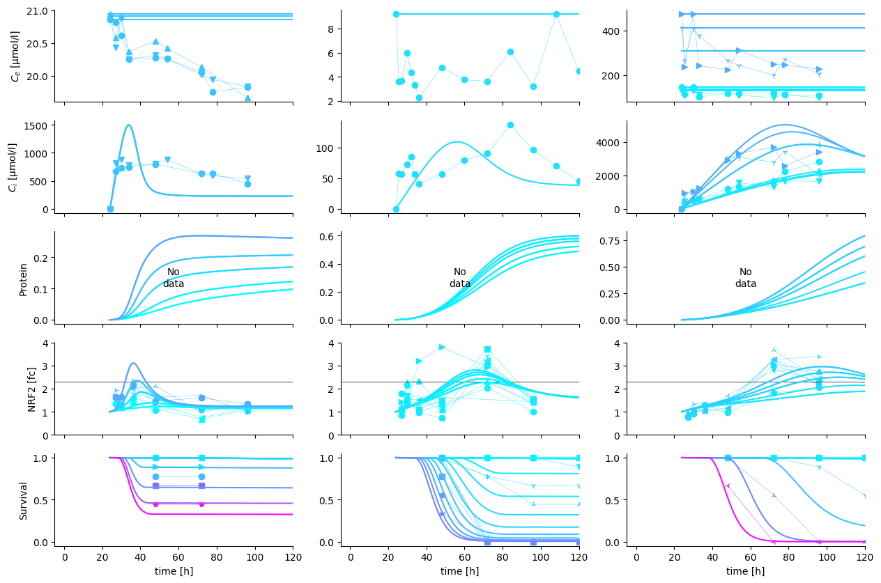
Next, we plot the predictions against selected experiments. Note that the observations, may be slightly diverging from the MAP predictions, because a) the model is not completely correct b) other data pull the posterior estimate away from the displayed data.
with open("../scenarios/rna_pulse_5_substance_independent_rna_protein_module/experiment_selection_1.json", "r") as fp:
    data_structure = json.load(fp)

res = res.assign_coords({"substance": sim.observations.substance})
cmap = mpl.colormaps["cool"]
fig, axes = plt.subplots(len(data_structure), 3, sharex=True, figsize=(15,10))


for r, (v, vdict) in enumerate(data_structure.items()):
    for c, (s, sdict) in enumerate(vdict["substances"].items()):
        sdata = sim.observations.where(sim.observations.substance == s, drop=True)
        C = np.round(sdata.cext_nom.values, 1)
        norm = mpl.colors.Normalize(vmin=C.min(), vmax=C.max())
        for eid in sdict["experiment_ids"]:

            ax, meta, obs_ids, _ = sim._plot.plot_experiment(
                self=sim,
                experiment_id=eid,
                substance=s,
                data_var=v,
                cmap=cmap,
                norm=norm,
                ax=axes[r, c]
            )

            if v != "survival":
                ax.set_xlabel("")

            if v == "P":
                ax.set_ylabel("Protein")
                ax.spines[["right", "top"]].set_visible(False)

            if v == "nrf2":
                ax.set_ylim(0, 4)
                # note that the thresholds are mixed up. Diuron and Diclofenac should swap
                z = sim.inferer.idata.posterior.z.mean(("chain", "draw")).values
                ax.hlines(z, -10, 120, color="black", lw=0.5)

            if c != 0:
                ax.set_ylabel("")

            l = ax.get_legend()
            if l is not None:
                l.remove()
            ax.set_title("")

            res_ids = sim.get_ids(res, {"substance": s, "experiment_id": eid})

            for i in res_ids:
                y = res.sel(id=i)
                ax.plot(res.time, y[v], color=cmap(norm(y.cext.isel(time=0))))
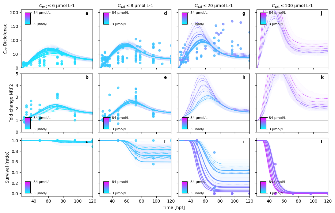
Posterior predictions#
In order to evaluate the goodness of fit for the posteriors, we are looking at the posterior predictions.
In order to obtain smoother trajectories, the time resolution is increased, and posterior predictions are calculated.
sim.config.inference.n_predictions = 100
sim.coordinates["time"] = np.linspace(24, 120, 200)
sim.seed=1
sim.config.data_structure.remove("lethality")
sim.dispatch_constructor()
_ = sim._plot.pretty_posterior_plot_multisubstance(sim, save=False, show=True)
Deleted 'lethality' DataVariable(dimensions=['id', 'time'] min=0.0 max=18.0 observed=False dimensions_evaluator=None).
PRETTY PLOT: starting...
Posterior predictions: 100%|██████████| 100/100 [00:08<00:00, 11.79it/s]
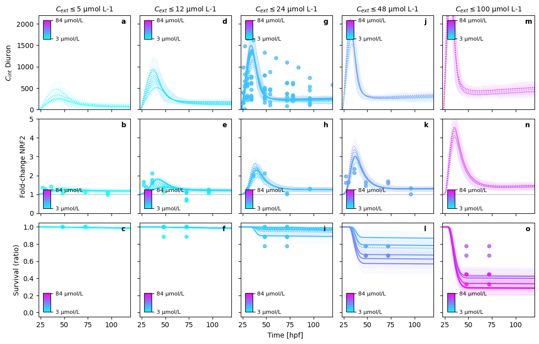
PRETTY PLOT: make predictions for Diuron in bin (1/5)
PRETTY PLOT: make predictions for Diuron in bin (2/5)
PRETTY PLOT: make predictions for Diuron in bin (3/5)
PRETTY PLOT: make predictions for Diuron in bin (4/5)
PRETTY PLOT: make predictions for Diuron in bin (5/5)
PRETTY PLOT: make predictions for Diclofenac in bin (1/4)
PRETTY PLOT: make predictions for Diclofenac in bin (2/4)
PRETTY PLOT: make predictions for Diclofenac in bin (3/4)
PRETTY PLOT: make predictions for Diclofenac in bin (4/4)
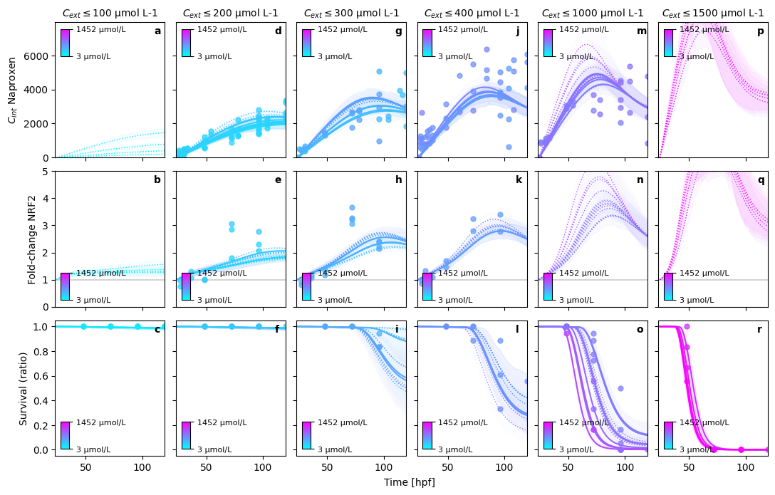
PRETTY PLOT: make predictions for Naproxen in bin (1/6)
PRETTY PLOT: make predictions for Naproxen in bin (2/6)
PRETTY PLOT: make predictions for Naproxen in bin (3/6)
PRETTY PLOT: make predictions for Naproxen in bin (4/6)
PRETTY PLOT: make predictions for Naproxen in bin (5/6)
PRETTY PLOT: make predictions for Naproxen in bin (6/6)